Download and install the UGENE NGS package to use this pipeline.
The ChIP-seq pipeline “Cistrome” integrated into UGENE allows one to do the following analysis steps: peak calling and annotating, motif search and gene ontology. ChIP-seq analysis is started from MACS tool. CEAS then takes peak regions and signal wiggle file to check which chromosome is enriched with binding/modification sites, whether bindings events are significant at gene features like promoters, gene bodies, exons, introns or UTRs, and the signal aggregation at gene transcription start/end sites or meta-gene bodies (average all genes). Then peaks are investigated in these ways:
- to check which genes are nearby so can be regarded as potential regulated genes, then perform GO analysis;
- to check the conservation scores at the binding sites;
- the DNA motifs at binding sites.
Note that it is originally based on the General ChIP-seq pipeline from the public Cistrome installation on the Galaxy workflow platform.
How to Use This Sample
If you haven't used the workflow samples in UGENE before, look at the "How to Use Sample Workflows" section of the documentation.
Workflow Sample Location
The workflow sample "ChIP-seq Analysis with Cistrome Tools" can be found in the "NGS" section of the Workflow Designer samples.
Workflow Image
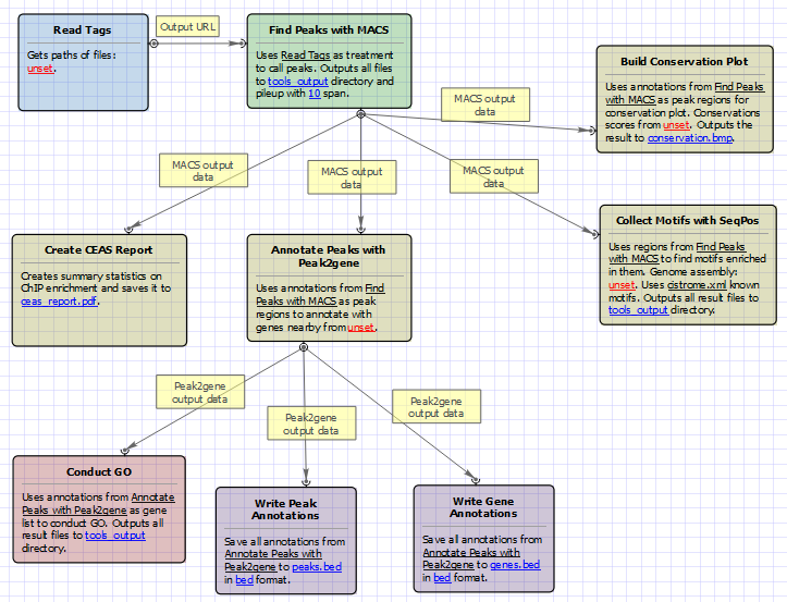
For treatment tags only analysis type the workflow looks as follows:
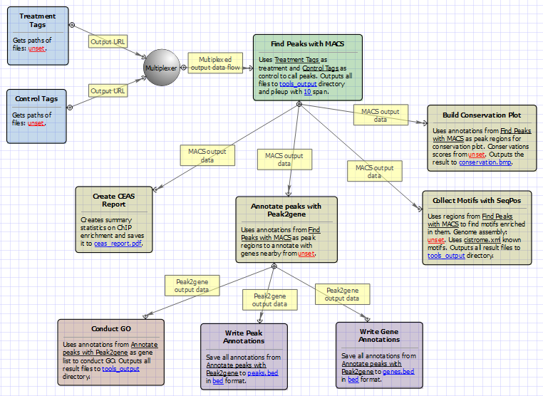
For treatment and control tags analysis type the workflow looks as follows:
Workflow Wizard
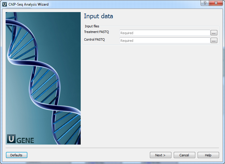
The wizards are the same for both types of workflows. The wizard has 7 pages.
Input data: Here you need to input a file with treatment and control annotations for MACS.
MACS: Here you can change default MACS parameters.
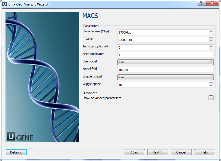
The following parameters are available:
Genome size (Mbp)
Homo sapience - 2700 Mbp
Mus musculus - 1870 Mbp
Caenorhabditis elegans - 90 Mbp
Drosophila melanogaster - 120 Mbp
It's the mappable genome size or effective genome size which is defined as the genome size which can be sequenced. Because of the repetitive features on the chromosomes, the actual mappable genome size will be smaller than the original size, about 90% or 70% of the genome size.
P-value
P-value cutoff. Default is 0.00001, for looser results, try 0.001 instead.
Tag size (optional)
Length of reads. Determined from first 10 reads if not specified (input 0).
Keep duplicates
It controls the MACS behavior towards duplicate tags at the exact same location -- the same coordination and the same strand. The default auto option makes MACS calculate the maximum tags at the exact same location based on binomal distribution using 1e-5 as pvalue cutoff; and the all option keeps every tags. If an integer is given, at most this number of tags will be kept at the same location.
Use model
Whether or not to use MACS paired peaks model.
Model fold
Select the regions within MFOLD range of high-confidence enrichment ratio against. Model fold is available when Use Model is true, which is the foldchange to chose paired peaks to build paired peaks model. Users need to set a lower(smaller) and upper(larger) number for fold change so that MACS will only use the peaks within these foldchange range to build model.
Wiggle output
If this flag is on, MACS will store the fragment pileup in wiggle format for the whole genome data instead of for every chromosomes.
Wiggle space
By default, the resolution for saving wiggle files is 10 bps, i.e., MACS will save the raw tag count every 10 bps. You can change it along with Wiggle output parameter.
Shift size
An arbitrary shift value used as a half of the fragment size when model is not built. Shift size is available when Use Model is false, which will represent the HALF of the fragment size of your sample. If your sonication and size selection size is 300 bps, after you trim out nearly 100 bps adapters, the fragment size is about 200 bps, so you can specify 100 here.
Band width
The band width which is used to scan the genome for model building. You can set this parameter as the sonication fragment size expected from wet experiment. Used only while building the shifting model.
Use lambda
Whether to use local lambda model which can use the local bias at peak regions to throw out false positives.
Small nearby region
The small nearby region in basepairs to calculate dynamic lambda. This is used to capture the bias near the peak summit region. Invalid if there is no control data.
Auto bimodal
Whether turn on the auto pair model process.If set, when MACS failed to build paired model, it will use the nomodelsettings, the Shift size parameter to shift and extend each tags.
Scale to large
When set, scale the small sample up to the bigger sample.By default, the bigger dataset will be scaled down towards the smaller dataset,which will lead to smaller p/qvalues and more specific results. Keep in mind that scaling down will bring down background noise more.
CEAS: The next page allows to configure CEAS parameters.
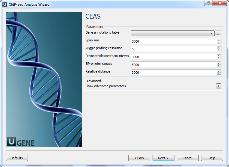
The following parameters are available:
Gene annotations table
Path to gene annotation table (e.g. a refGene table in sqlite3 db format.
Span size
Span from TSS and TTS in the gene-centered annotation (base pairs). ChIP regions within this range from TSS and TTS are considered when calculating the coverage rates in promoter and downstream.
Wiggle profiling resolution
Wiggle profiling resolution. WARNING: Value smaller than the wig interval (resolution) may cause aliasing error.
Promoter/downstream interval
Promoter/downstream intervals for ChIP region annotation are three values or a single value can be given. If a single value is given, it will be segmented into three equal fractions (e.g. 3000 is equivalent to 1000,2000,3000).
BiPromoter ranges
Bidirectional-promoter sizes for ChIP region annotation. It's two values or a single value can be given. If a single value is given, it will be segmented into two equal fractions (e.g. 5000 is equivalent to 2500,5000).
Relative distance
Relative distance to TSS/TTS in WIGGLE file profiling.
Gene group files
Gene groups of particular interest in wig profiling. Each gene group file must have gene names in the 1st column. The file names are separated by commas.
Gene group names
Set this parameter empty for using default values.
The names of the gene groups from "Gene group files" parameter. These names appear in the legends of the wig profiling plots.
Values range: comma-separated list of strings. Default value: 'Group 1, Group 2,...Group n'.
Peak2Gene and Gene Ontology: The next page allows to configure Peak2Gene and Gene Ontology parameters.
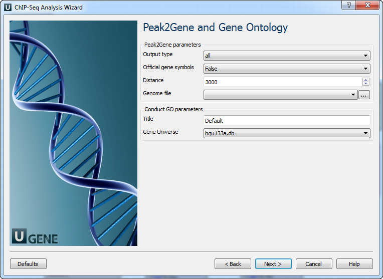
The following parameters are available:
Output type
The directory to store Conduct GO results.
Official gene symbols
Output official gene symbol instead of refseq name.
Distance
Set a number which unit is base. It will get the refGenes in n bases from peak center.
Genome file
Select a genome file (sqlite3 file) to search refGenes.
Title
Title is used to name the output files - so make it meaningful.
Gene Universe
Select a gene universe.
Conservation plot: On this page you can modify Conservation Plot parameters.
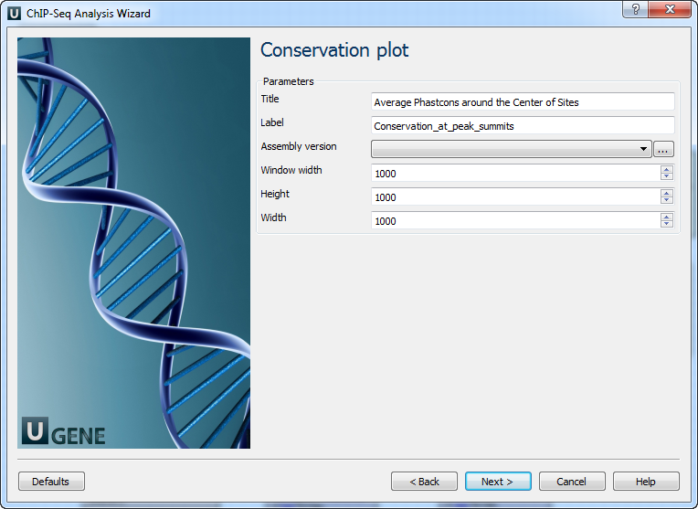
The following parameters are available:
Title
Title of the figure.
Label
Label of data in the figure.
Assembly version
The directory to store phastcons scores.
Window width
Window width centered at middle of regions.
Height
Height of plot.
Width
Width of plot.
SeqPos motif tool: On this page you can modify SeqPos motif parameters.
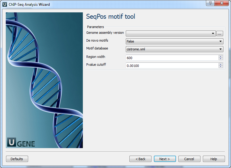
The following parameters are available:
Genome assembly version
UCSC database version.
De novo motifs
Run de novo motif search.
Motif database
Known motif collections.
Region width
Width of the region to be scanned for motifs; depends on a resolution of assay.
Pvalue cutoff
Pvalue cutoff for the motif significance.
Output data: On this page you can modify output parameters.
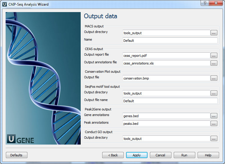
The following parameters are available.
MACS output:
Output directory
Directory to save MACS output files.
Name
Name string of the experiment. MACS will use this string NAME to create output files like 'NAME_peaks.xls', 'NAME_negative_peaks.xls', 'NAME_peaks.bed', 'NAME_summits.bed', 'NAME_model.r' and so on. So please avoid any confliction between these filenames and your existing files.
CEAS output:
Output report file
Path to the report output file. Result for the CEAS analysis.
Output annotations file
Name of tab-delimited output text file, containing a row of annotations for every RefSeq gene. Note that the file is not generated if there is no peak regions input.
Conservation Plot output:
Output file
File to store phastcons results (BMP).
SeqPos motif tool output:
Output directory
Directory to store seqpos results.
Output file name
Name of the output file which stores new motifs found during a de novo search.
Peak2Gene output:
Gene annotations
Location of peak2gene gene annotations data file.
Peak annotations
Location of peak2gene peak annotations data file.
Conduct GO output:
Output directory
Directory to store Conduct GO results.
The work on this pipeline was supported by grant RUB1-31097-NO-12 from NIAID.